Simulation Learning Log

What is Simulation?

Table of Contents

1. Background
2. Tragedy of the Commons
   • Modeling
3. Causal Loop Diagram
   • Components
   • Types of Loops
   • Delays
4. System Archetype
   • Escalation
   • Success to Successful
5. From Causal Loop Diagram to System Dynamics Model
   • Key Steps
   • Example: Population Growth Model
6. Simulation Time Flow and Finite State Machine
   • Simulation Time Flow
   • Finite State Machine
     • Key Components
     • Characteristics
     • Example: Vending Machine
   • Applications in Simulation

Background

In this article, we will explore the basics of simulation and modeling. What is simulation? According to Claude, my favorite AI assistant, simulation is the imitation of real-world systems, states, or processes through computer or physical models. Wouldn’t it be incredibly useful if we could predict the real world through simulation?

This article is primarily based on the online open course Introduction to Modeling and Simulation from KAIST.

Tragedy of the Commons

There are various public resources in the world. Notable examples include water, land, and oil. The tragedy of the commons refers to the economic and scientific situation where these shared resources, if not managed separately and consumed by individuals according to their own interests, will be depleted. This example is often used to explain simulation and modeling.

Let’s consider a scenario. There are two shepherds, each with their own flock of sheep. They are in a competitive relationship. Given that the pasture where the sheep can graze is limited, what choices should the shepherds make to maximize their own benefits?

1. Let the sheep graze all day.
2. Increase the size of the flock.

While there are various choices, ultimately, the faster and more one consumes the shared resource (pasture) compared to the competitor, the more their benefits are maximized. If limited public goods are consumed through such choices, the result will inevitably be depletion.

Modeling

How can we model this example? Let’s first define the important objects:

1. Pasture
2. Flock of sheep
3. Shepherd
4. Barren land

But unfortunately, this is not the end. We also need to define the attributes and relationships of each object:

1. Rate of change from pasture to barren land based on flock size
2. Rate of change from barren land to pasture over time
3. Reproduction rate of the flock
4. Total size of the pasture

The attributes/relationships defined here are just a part of what needs to be considered. There are many more factors to take into account.

Causal Loop Diagram

A causal loop diagram is a tool for visually representing the causal relationships between variables in a system. It uses arrows to show relationships between variables, distinguishing between positive (+) and negative (-) relationships. When modeling for simulation, using a Causal Loop Diagram allows you to observe an abstracted view of the model.

There are three main components in a Causal Loop Diagram:

1. Factors
   • Factors are numerical variables that represent quantity or intensity.
2. Relationships between the factors
   • Relationships include feedback and positive/negative links.
3. Delays
   • We’ll explain delays in more detail later.

Positive/negative links can create loops, and there are two types of loops:

• Reinforcing loop
  • A reinforcing loop occurs when the number of negative links in the cycle is even.

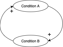
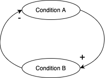
• Balancing loop
  • A balancing loop occurs when the number of negative links is odd.

Delays

Without delays, modeling can be simplified and made to work ideally. However, most real-world problems include delays.

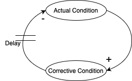
For example, if you keep placing orders because products haven’t arrived, you might end up with more products than expected. To resolve this, you might return some, but returns also have delays, which can cause similar problems as with the orders. This is called oscillations.
If the oscillations converge to the target value, the goal can be achieved, but if the error keeps growing, this is called the bullwhip effect. This is a common problem that can occur in supply chain management (SCM).

System Archetype

A system archetype is a conceptual model that describes recurring behavior patterns in organizations or systems. Understanding archetypes can help more easily identify and solve problems in complex systems.

You can find images and more detailed explanations of the examples below at System Archetype.

Archetype: Escalation

This type includes scenarios like the chicken game and arms races. There is a common factor between two loops, and this factor controls both loops. For example, if country A increases its military power, country B also needs to increase its military power, resulting in a continuous escalation effect on both sides.

Archetype: Success to Successful

This type explains the phenomenon where, in a situation with limited resources, when there are A and B, as more resources are invested in A, B’s power weakens. Both loops are reinforcing loops, but they go in different directions.

From Causal Loop Diagram to System Dynamics Model

While Causal Diagrams were good for conceptually modeling scenarios, they pose challenges in terms of complexity and visibility when modeling actual complex problems. In other words, to develop from a qualitative model to a quantitative model, we need to evolve into a System Dynamics Model. This process includes mathematical definition of variables, setting initial values, and equation formulation.

Key Steps:

1. Variable Identification and Definition:
   • Define each element of the causal loop diagram as a clear variable.
   • Determine the type of each variable (stock, flow, auxiliary).
2. Establishing Mathematical Relationships:
   • Express the relationships between variables as mathematical equations.
   • Example: Population growth rate = Birth rate - Death rate
3. Setting Initial Values:
   • Define the initial values for each stock variable.
   • Represents the system state at the start of the simulation.
4. Setting Time Units and Simulation Period:
   • Decide on the time unit of the model (e.g., day, month, year).
   • Set the overall simulation period.
5. Defining Functions and Tables:
   • Create graph functions or lookup tables to express non-linear relationships.
6. Implementing Feedback Loops:
   • Convert the feedback structure of the causal loop diagram into mathematical relationships.
7. Modeling Delay Effects:
   • Use appropriate delay functions to express the system’s delay effects.

Example: Population Growth Model

You can find additional images and examples at System Dynamics.

Causal loop diagram:

Birth rate (+) --> Population --> (+) Birth rate
Population --> (+) Death rate --> (-) Population

System dynamics model:

Population(t) = Population(t-dt) + (Birth rate - Death rate) * dt
Initial Population = 1000
Birth rate = Population * Birth_rate_coefficient
Death rate = Population * Death_rate_coefficient
Birth_rate_coefficient = 0.03
Death_rate_coefficient = 0.02

Simulation Time Flow and Finite State Machine

In simulation, time can be modeled as continuous or discrete. A finite state machine is a model where the system has a finite number of states and transitions between states occur according to specific conditions.

These two concepts play important roles in modeling the dynamic behavior of various systems.

Simulation Time Flow

There are two main ways to model the flow of time in simulations:

1. Continuous Time Flow:
   • Models time as flowing continuously without interruption.
   • Uses differential equations to express changes in the system.
   • Examples: Physical systems, chemical reactions, population dynamics, etc.
2. Discrete Time Flow:
   • Models time in discrete intervals.
   • Uses difference equations or discrete events to express changes in the system.
   • Examples: Digital systems, production lines, computer networks, etc.

The choice of time flow depends on the characteristics of the system being modeled and the purpose of the simulation.

Finite State Machine

A finite state machine is a mathematical model that represents the behavior of a system as a finite number of states and transitions between them.

Key Components

1. States: All possible conditions or situations the system can be in
2. Transitions: Changes from one state to another
3. Events: Conditions or inputs that trigger transitions
4. Actions: Operations performed during state changes

Characteristics

• Clarity: Can clearly define the behavior of the system.
• Predictability: Can easily predict the system’s response to given inputs.
• Ease of Testing: Can individually test each state and transition.

You can find additional images and examples at Finite State Machine.

Example: Vending Machine

States: Waiting, Selection, Payment, Dispensing
Transitions:
  Waiting -> Selection (Product button pressed)
  Selection -> Payment (Money inserted)
  Payment -> Dispensing (Payment completed)
  Dispensing -> Waiting (Product dispensed)

Applications in Simulation

1. Modeling Complex Systems:
   • Hybrid modeling is possible by combining continuous and discrete concepts.
   • Can use finite state machines to define the main behaviors of the system.
2. Event-Based Simulation:
   • Can implement event-centered simulations by combining discrete time flow and finite state machines.
3. System Verification:
   • Can systematically verify all possible states and transitions of the system through finite state machines.
4. Real-Time System Design:
   • Can model physical processes using continuous time flow and implement control logic with finite state machines.